Creating a GPF Graph

This tutorial shows how multiple Graph Processing Framework (GPF) operators can be combined to a graph.
This allows to perform multiple operations in a chain.

Not all options and features are covered in this tutorial, but it gives a brief overview of the capabilities of GPF.
The example is made with a Windows command-line for Linux and Mac Os X you have to adopt the calls appropriately.
If questions arise please consult the SNAP Forum

Introduction to gpt

To get familiar with GPF, let's have a look at the GPF related command line tool named gpt.

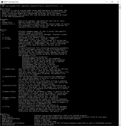
Open a console window at $SNAP_INSTALL_DIR$/bin and type: gpt -h.
This will print out a short description of what the tool is good for and describes the arguments and options of the tool. Also a list of public available operators is displayed.

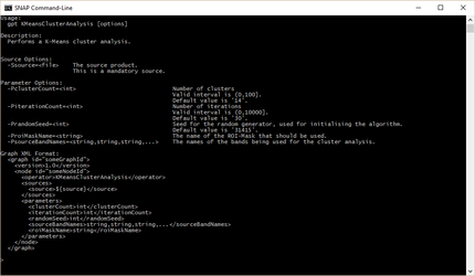
The usage text for a concrete operator can be displayed by executing gpt $OperatorName$ -h.
In the following image the usage text for the KMeansClusterAnalysis operator is printed.

The usage text of an operator also displays a template clipping of the operators configuration when used in a graph.

Creating a First Graph

As a first example we will create a graph with only a single operator.
We use the BandMaths operator to extract the flag CLDICE from a MODIS Ocean Color L2 data product.

<graph id="firstGraph">
   <version>1.0</version>
     <node id="cloudNode">
       <operator>BandMaths</operator>
       <sources>
           <sourceProducts>${sourceProducts}</sourceProducts>
       </sources>
       <parameters>
           <targetBands>
               <targetBand>
                   <name>cloudMask</name>
                   <expression>l2_flags.CLDICE</expression>
                   <description>Cloud mask derived from l2_flags</description>
                   <type>int32</type>
                   <noDataValue>NaN</noDataValue>                   
               </targetBand>               
           </targetBands>
       </parameters>
   </node>
</graph>

Put the xml in a file named cloudMask.xml. And now type at the command line:
gpt c:\tutorial\cloudMask.xml -t c:\tutorial\out\mask.dim C:\tutorial\in\A2008112121000.L2_LAC.hdf
The first argument specifies the graph file to be used for processing, the -t option specifies the target file where the result is written to, and the last argument specifies the source product for processing.

You might have noticed that in the list of available operators a Read and a Write operator exist. Now you might wonder why these are not used in the graph. The answer is they are not needed. GPF is smart enough to add those operators to the graph on its own. You have to declare them in the graph only in some special cases. But we will not cover these cases in this simple tutorial.

Multiple Operator Graph

Now, we will create a more sophisticated graph.
The task is to create a cloud mask derived from flags, reproject the source product to UTM and write only some bands to the target product.
Therefore we use the BandMaths operator to create the cloud mask band and also to copy bands we like to have in the target product. Afterwards the Reproject operator is used to reproject the product to UTM CRS. Finally we use the subset op in order to limit the band set to the ones we like to have.

<graph id="cloud_reproj_subset">
   <version>1.0</version>
     <node id="cloudNode">
       <operator>BandMaths</operator>
       <sources>
           <sourceProducts>${sourceProducts}</sourceProducts>
       </sources>
       <parameters>
           <targetBands>
               <targetBand>
                   <name>cloudMask</name>
                   <expression>l2_flags.CLDICE</expression>
                   <description>Cloud mask derived from l2_flags</description>
                   <type>int8</type>
                   <noDataValue>NaN</noDataValue>                   
               </targetBand>               
               <targetBand>
                   <name>nLw_443</name>
                   <expression>nLw_443</expression>
                   <description>Normalized water-leaving radiance at 443 nm</description>
                   <type>float32</type>
                   <validExpression></validExpression>
                   <noDataValue>0.0</noDataValue>
                   <spectralBandIndex>0</spectralBandIndex>
                   <spectralWavelength>443.0</spectralWavelength>
                   <spectralBandwidth>0.0</spectralBandwidth>
               </targetBand>
               <targetBand>
                   <name>chlor_a</name>
                   <expression>chlor_a</expression>
                   <description>Chlorophyll Concentration, OC3 Algorithm</description>
                   <type>float32</type>
                   <validExpression>(chlor_a >= 0 and chlor_a &lt;= 100)</validExpression>
                   <noDataValue>NaN</noDataValue>
               </targetBand>
           </targetBands>
       </parameters>
   </node>

   <node id="reprojNode">
       <operator>Reproject</operator>
       <sources>
           <source>cloudNode</source>
       </sources>
       <parameters>
           <!-- UTM Automatic -->
           <crs>AUTO:42001</crs>
           <resampling>Nearest</resampling>
           <includeTiePointGrids>false</includeTiePointGrids>
       </parameters>
   </node>
   
   <node id="subsetNode">
       <operator>Subset</operator>
       <sources>
           <source>reprojNode</source>
       </sources>
       <parameters>
           <bandNames>cloudMask,chlor_a,nLw_443</bandNames>
           <copyMetadata>true</copyMetadata>
       </parameters>
   </node>
</graph>

Here the operators are concatenated by specifying the preceding node id as source of the current node.
The first node (cloudNode) of the graph uses the BandMaths operator we already know. it is configured to create the cloudMask band and also to copy the bands nLw_443 and chlor_a. The second node (reprojNode) reprojects the output of the cloudNode to the UTM coordinate reference system. The last one (subsetNode) creates a band subset from the output of the reprojNode. It ensures that only the three specified bands (cloudMask,chlor_a,nLw_443) are written to the target product.