Product Data Model
- Former user (Deleted)
- Marco Peters
- Nicolas Ducoin (Unlicensed)
- Tonio Fincke
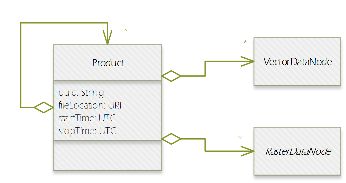
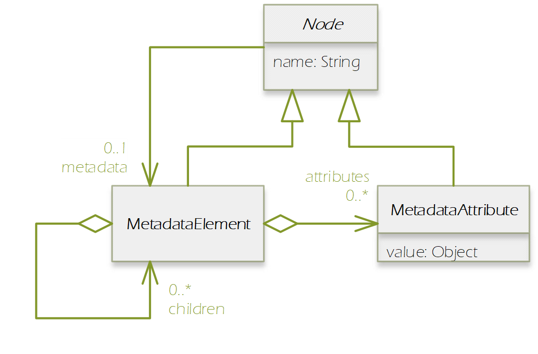
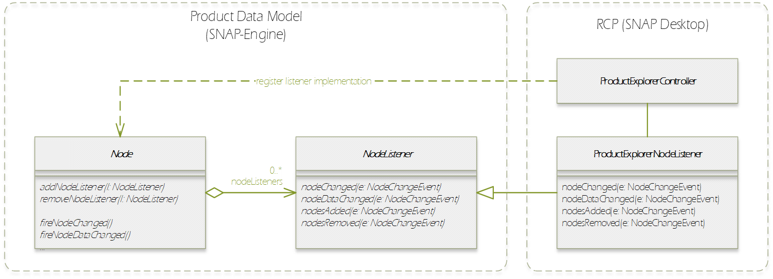
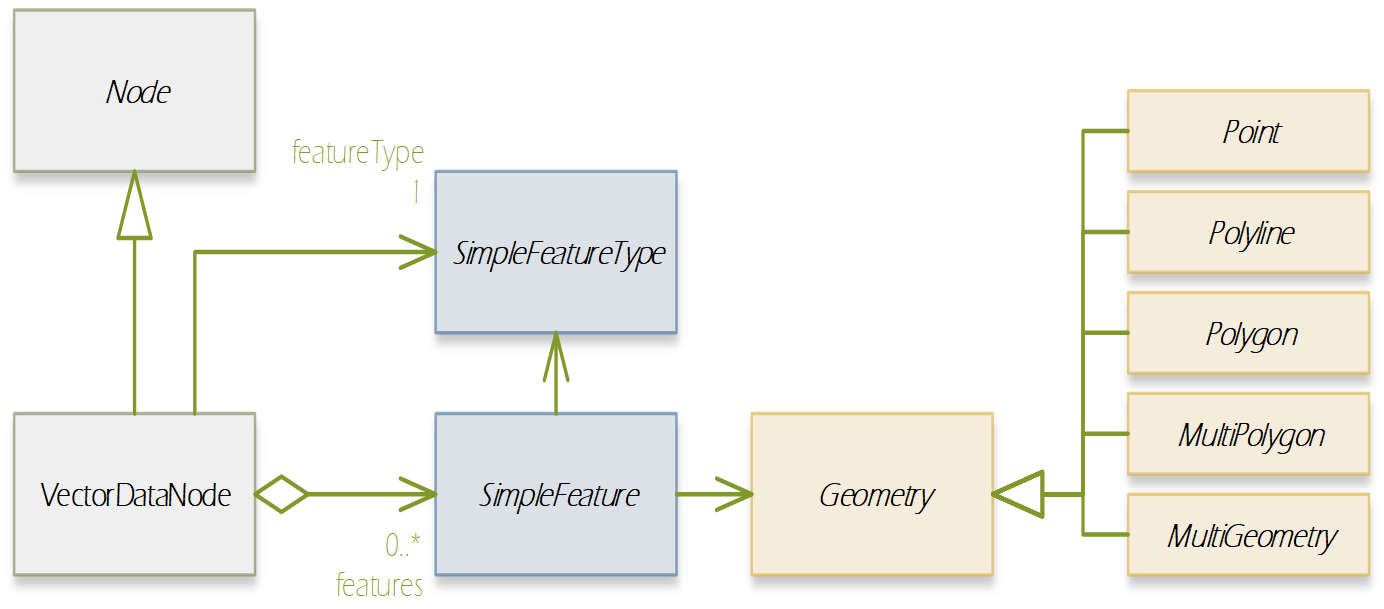
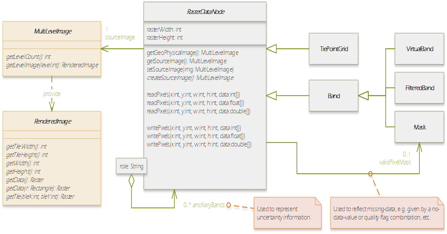
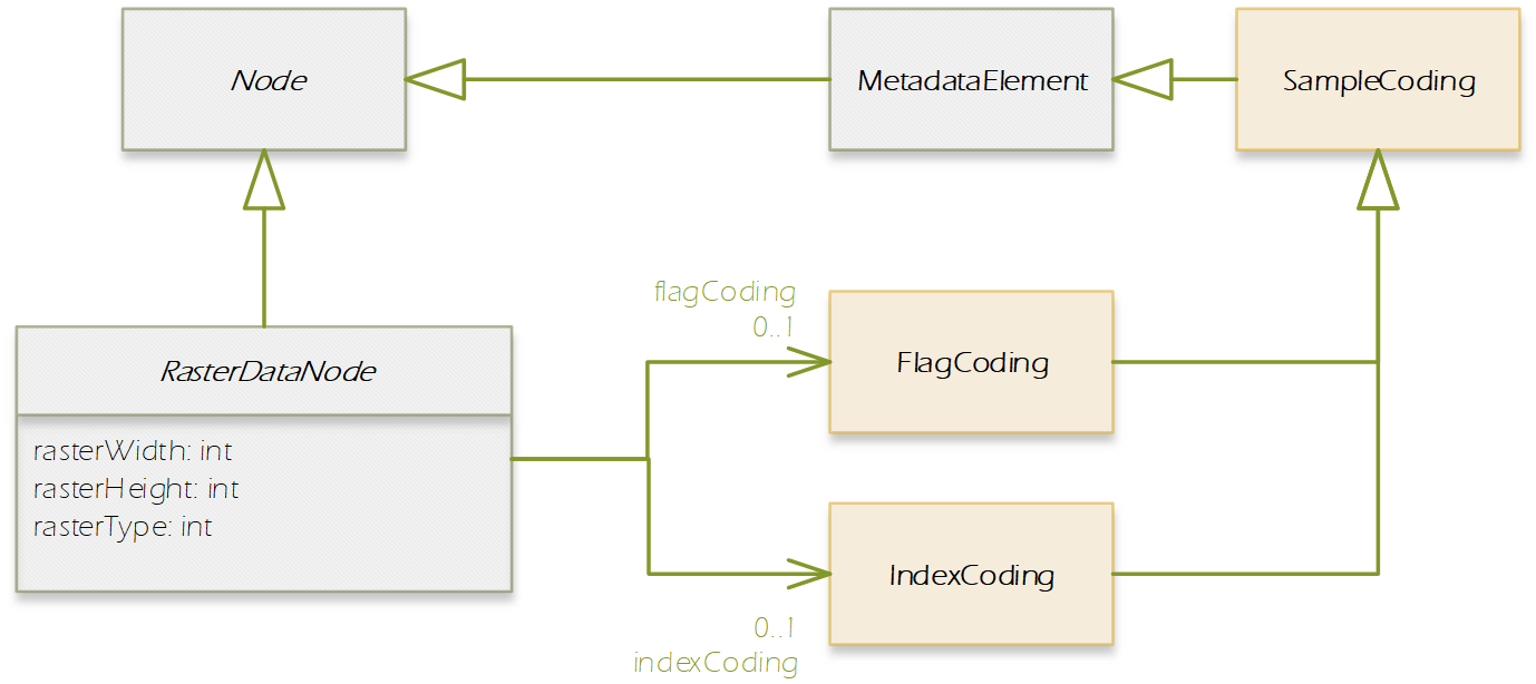
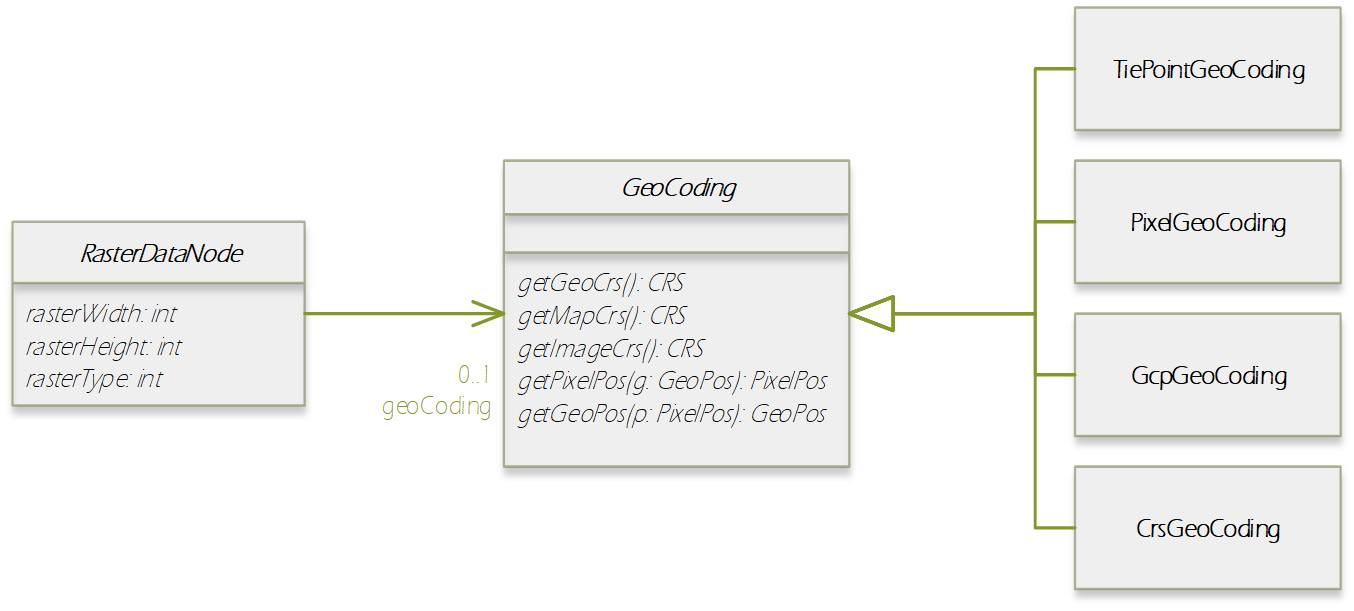
In this section, we introduce the Product Data Model (PDM) of SNAP which is applicable to a large variety of remote sensing data. The PDM is the central concept in the Sentinel Toolbox as it provides an abstraction from the actual data formats from which EO data is read and written to. The PDM is accessible to developers by a dedicated API which provides an interface to a variety of data sources and which hides the details of the internal data management (e.g. in-memory tile caching, local file caching of remote data). Specific data I/O issues are fully transparent to developers of data processor and data writer plugins. They just use the PDM API to implement their algorithms or data format encodings. The same holds true for developers of new GUI components, visualisations, analyses, plots and other plug-ins. They are all independent of whatever data products are supported or any specific complexities of the file formats (the applicability is restricted where a processing function expects specific product contents). Format conversions from one file format to another are easily achieved with the available data reader and data writer plugins. The SNAP PDM can In the following, we will explain aspects of the PDM using UML class diagrams. The first conceptual diagram introduces the Product class which represents an (EO) data product containing both vector data represented by a VectorDataNode collection and raster data represented by a RasterDataNode collection. (Collections are indicated by a diamond on the provider side and a multiplier asterisk [*] on the item side of the relationship connector.). The diagram also indicates that each product contains its file location (if any) in form of a Universal Resource Locator (URI), and its start/stop sensing/aggregation time in form of a UTC timestamp: Every Node can have (as indicated by the 0..1 multiplier) metadata represented by a MetadataElement associated with it. A MetadataElement can have any number of other MetadataElement children and have a MetadataAttribute collection, which can carry the actual values (of any type). This model reflects metadata as it may be externally represented in XML (ESA SAFE format, DIMAP, GML), or NetCDF, HDF or also JSON. Both the MetadataElement and MetadataAttribute class are a Node (as indicated by the triangle symbol in their relationship connectors). When we refer to a node collection we are actually referring to a relationship modelled by the Group class (collection design pattern). It maintains a list of Node children and is also a Node. Any node can only be contained in at most one Group which is reflected by its parent property. Using the Group class, we can model possible multi-dimensionality (depth, pressure, time) of VectorDataNodes and RasterDataNodes which usually have the two (geo-) spatial dimensions x and y (or longitude and latitude) in a coordinate reference system. The SNAP Desktop GUI must be responsive to any change in a PDM instance. Multiple GUI components may refer to same PDM instance parts, such as displayed raster data images, names in titles, or metadata tables. In order to immediately reflect any change in a PDM instance in all of these GUI components, the PDM must be observable. The following diagram shows that a Node also has a NodeListener list. A NodeListener is an abstract interface that is implemented by (client) classes wishing to be informed about changes in a node. If a node changes, it informs its NodeListers about that change. In the diagram, the ProductExplorerController as part of some GUI module, registers its listener implementation in a Product (Node) in order to update the GUI on any Node change. Node changes are hierarchical. Any child node will also inform its parent node about the change. Vector data, such as data loaded from ESRI shape files or from GML is represented by a VectorDataNode. A VectorDataNode comprises a SimpleFeature collection. A feature is basically a container of attributes (key-value pairs) according to a given schema, the SimpleFeatureType which describes order, name, and value type of all the attributes. At least one of the attributes represents the feature’s geometry, its location/extent on the Earth’s surface. Geometries can be of any 1D/2D type as indicated by the diagram. For the CDM, we use the SimpleFeature API as specified by ISO 19125-1:2004 [http://www.iso.org/iso/catalogue_detail.htm?csnumber=40114] and implemented by the GeoTools 3rd party library [http://www.geotools.org/]. Non-geometry attributes may have any data type and are used to represent geophysical measurements, classification or statistical data. As VectorDataNode instance can also be used to store geometry created by a Sentinel Toolbox user. SNAP uses VectorDataNodes to store pins, ground-control-points, and any shape figures (e.g., polylines used as transects) drawn by the user. As mentioned before, the RasterDataNode class is used to represent 2D raster data of any numerical data type. Within the PDM, raster data can accessed via the RasterDataNode class in two ways. The first approach is straight forward: API users can directly call various readPixel() methods on an instance, from which they obtain geophysical pixel values (scaled by scaling factor, offset, with no-data indicated as NaN values). Users provide raster region in pixel coordinates and the data array to receive the pixel values. The second approach is more advanced as it makes advantage of the actual internal storage model for large raster datasets, namely pyramids of tiled images which are represented by the MultiLevelImage class shown in the following diagram. MultiLevelImage instances exist for the raw, source raster data and the scaled, geophysical raster data. MultiLevelImages compute their raster data tiles on-the-fly and not before a tile is requested, e.g., for display or processing. RasterDataNodes can contain references to ancillary RasterDataNodes via roles, e.g. “uncertainty”, “confidence”, or “probability”. SNAP provides multiple visualisation modes (overlay, blending) for such ancillary raster data. Multiple sub-classes of RasterDataNodes exist which basically differ in the way their source image (MultiLevelImage) instances are created and how they receive/generate their raster data. Some bands provide raster data whose pixels are integer numbers which again are binary representations of quality flag information. An associated FlagCoding class is used to describe the flags in such an integer. FlagCoding instances are metadata element whose attributes are the single flags, e.g., “INVALID” may have the mask value “0x02”. Very similar to FlagCoding, an IndexCoding is used to describe and interpret integer pixel values in terms of an index. The GeoCoding interface is an abstraction of how to obtain geographical coordinates from a raster’s pixel coordinates and vice versa: Various implementations of the GeoCoding interface exist. The most frequently used ones are: